Can Orange explore a 13 GB data set?

What was the largest file you ever worked with in Orange? Mine used to be a 2D spectral image of about 2 GB. I got it from a colleague to stress-test visualizations in the Spectroscopy add-on. At that time, in 2018, I only had a laptop with 8 GB of working memory, so, apart from the stress tests, I could not do much with it. Running machine learning techniques was a no-go because intermediate results immediately filled my memory. Furthermore, in Orange, even simple operations such as normalization can multiply data in memory; after that, Orange needs twice the space because it also needs to store both the original and the normalized data.

Things change. My current laptop has 16 GB of memory. But more importantly, my Orange version has a trick up its sleeve: support for on-disk data. Yours could support it, too, but you'll need to use Orange from the experimental dask branch. Installation is not for the faint-hearted, but if you are curious about testing these features, follow our installation guide.

To see how it works, we will use a data set of tissue sections of breast cancer. The data set BRC961-BR1001 was shared by David Mayerich. Originally, it was even larger than 100 GB, so we took a subset and converted it into a special HDF5 format that Orange can read with Dask. We obtained a 13 GB HDF5 file; you can download it here.

When we load brc961-br1001-orange.hdf5 with the File widget, it loads immediately! What? Whoever used Orange with even slightly bigger data will know loading files takes time. But here, with 13 GB, it was immediate! That is, well, because almost nothing happened: the file was loaded with Dask, meaning only its metadata was read, but the actual content was not read. With Dask, the paradigm is that data is only accessed when needed. We can observe that if we connect Data Table and scroll around. After scrolling, we see a slight delay before data is shown: only now the actual values are read (for a longer story about, see Noah's blog).

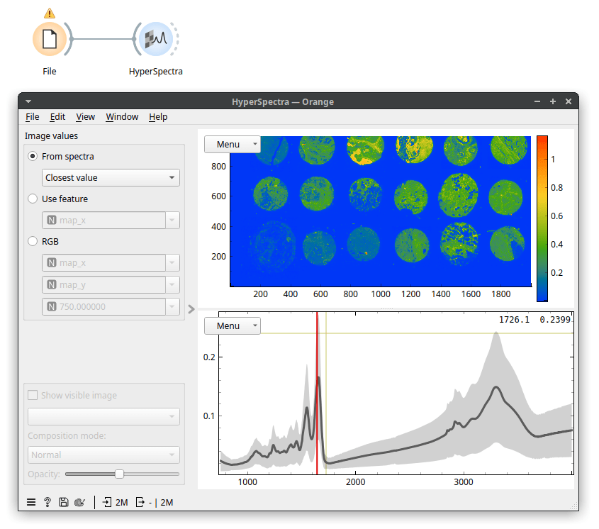
Because our data is a spectral map, we view it in the HyperSpectra widget. I've set the widget to color by values of the Amide I peak (wavenumber 1650). On my laptop, it takes about a minute for the HyperSpectra to show both plots fully. Now, the data was being read but was only read in chunks, so it did not fill up our working memory. In the map, we see 18 tissue sections on a microscope slide. The slide contains no useful information, so we can remove it. It has low values for wavenumber 1650 (the Amide I peak). Let's use Distributions to plot that.

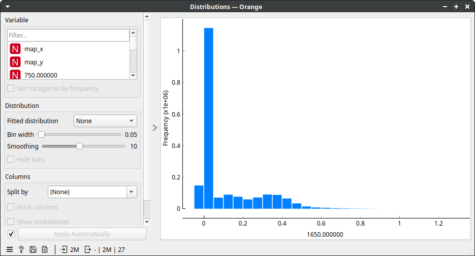
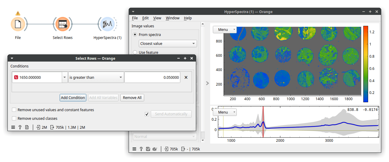
That took a while, but a useful cutoff seems to be somewhere between 0 and 0.2. Therefore, let's be conservative and instruct Select Rows to select rows with wavenumber 1650 higher than 0.05. Now, we see the following.

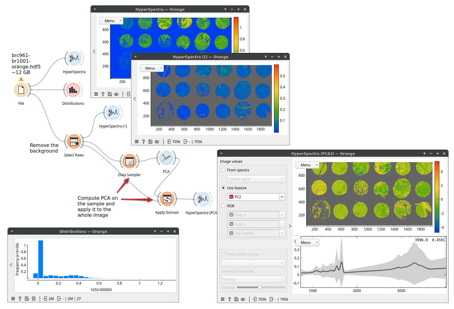
Next, let's perform principal component analysis (PCA). Because PCA is computationally more demanding, we will use Data Sampler to run PCA on a subset of 10000 rows (spectra). Then, we will apply (with Apply Domain) the computed principal components to the whole data set and view the resulting PCA scores as an image. Here, we show the full workflow.

Because only a subset of Orange's widget supports Dask (basic data manipulation and simpler machine learning techniques, for example, k-Means, Linear Regression, Logistic Regression) we may need to escape it. Fortunately, there is a way: the Dask Compute widget brings a table to memory. Performance-wise, it always makes sense to work in memory if we can afford it. Here, we selected one tissue sample, stored it in memory with Dask Compute, and can now work with this data that should be about 0.5 GB in size.

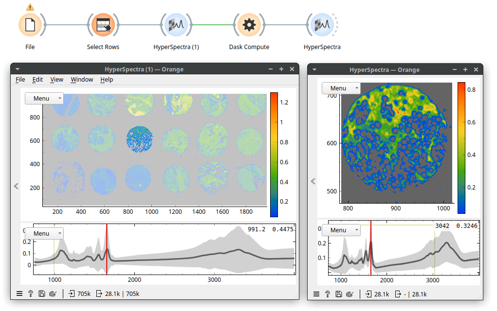
That's it! To try this yourself, install the experimental Orange version from the dask branch. And remember, start experimenting with smaller files.

Finally, we would like to thank the Chan Zuckerberg Initiative, which supported the development of Orange for big data.